Variance Reduction in Experiments, Part 1 - Intuition

The Difference-in-Means Estimator

Let’s consider the example, where our marketing team wants to figure out the impact of sending an email promotion. As a team of marketing data scientists, we decide to run an experiment by selecting 2000 random customers from our customer base. Our response variable is the amount of spending in the two weeks following the email, and for every customer, we let a coin flip decide whether that customer receives the promotion or not.

Since the treatment is delivered at random, we have no systematic bias, and a simple difference in means (DIM) between the treated (T) and control (C) in our experiment is an unbiased estimate of the population average treatment effect (ATE):

The critical point here is that this estimator gives us the true effect on average, but for a given sample that we end up analyzing, it might as well be far away from it.

In the following code we first generate a sample of 2000 customers, randomly select half of them to treatment that has a constant effect of $5 on customer spending. We then apply the DIM estimator using linear regression on this sample, hoping to recover the true effect.

def dgp(n=2000, p=10):
        
    Xmat = np.random.multivariate_normal(np.zeros(p), np.eye(p), size=n).astype('float32')

    T = np.random.binomial(1, 0.5, n).astype('int8')

    col_list = ['X' + str(x) for x in range(1,(p+1))]

    df = pd.DataFrame(Xmat, columns = col_list)
    
    # functional form of the covariates
    B = 225 + 50*df['X1'] + 5*df['X2'] + 20*(df['X3']-0.5) + 10*df['X4'] + 5*df['X5']

    # constant ate
    tau = 5 
    
    Y = (B + tau*T + np.random.normal(0,25,n)).astype('float32')
        
    df['T'] = T
    df['Y'] = Y

    return df

data = dgp()
ols = smf.ols('Y ~ T', data = data).fit(cov_type='HC1',use_t=True)
ols.summary().tables[1]

Unfortunately, the DIM estimate for this particular sample is far away than the true effect and is negative in sign. It also comes with a quite wide confidence interval, which prevents us from drawing any conclusions.

On the other hand, if we had the opportunity to repeat this experiment thousands of times in parallel with a different sample of the population each time, we would see that the density of our estimates would peak around the true effect. To see this, let’s create a simulation that generates a sample of 2000 customers and runs the previous experiment every time it is called, for 10000 times.

def experiment(**kwargs):
    dct = {}
    
    n = kwargs['n']
    p = kwargs['p']
   
    df = dgp(n,p)
   
    #Difference-in-means
    mu_treated = np.mean(df.query('T==1')['Y'])
    mu_control = np.mean(df.query('T==0')['Y'])
    
    dct['DIM'] = mu_treated - mu_control

    return dct

def plot_experiment(results):
    results_long = pd.melt(results, value_vars=results.columns.tolist() )  
    mu = 5
    p = (ggplot(results_long, aes(x='value') ) + 
     geom_density(size=1, color='salmon')+
     geom_vline(xintercept=mu, colour='black', linetype='dashed' ) + 
     annotate("text", x=mu, y=.1, label="True Mean", size=15)+
     labs(color='Method')  +
     xlab('Estimate') +
     theme(figure_size=(10, 8))
    )
    return p

%%time
tqdm._instances.clear() 
sim = 10000
results = Parallel(n_jobs=8)(delayed(experiment)(n=2000, p=10)\
                                    for _ in tqdm(range(sim)) )

results_df = pd.DataFrame(results)
plot = plot_experiment(results_df)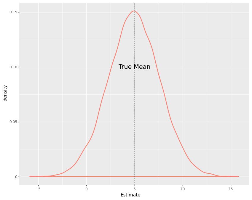

Variation in the Outcome

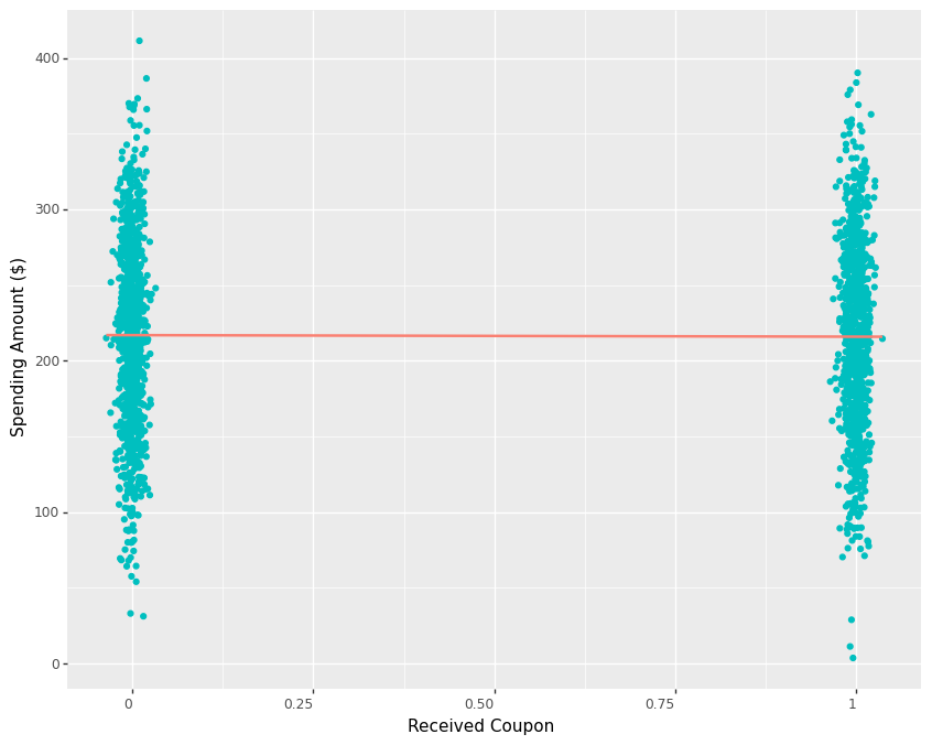
To understand why we fail to uncover the treatment effect when it is in fact present, we need to think about what actually determines customer spending. If our email promotion only has a limited impact in customer spending compared to other factors such as income, tenure with the business, recency, frequency and value of previous purchases etc. then it would be no surprise to see the variation of spending being explained much more by factors other than our email promotion. In fact, plotting customer spending against the treatment indicator reveals how it varies from around $4 to more than $400. Since we know that the promotion only has a small effect on spending, it becomes quite challenging to detect it inside all the variation. Hence, the regression line from control to treatment has a slight negative slope below.

One way we can make it easier for the DIM estimator to detect the true effect is by increasing our sample size. If we have access to, say 10000 customers instead of 2000, we can get a much closer estimate of the true effect as shown below.

data = dgp(n=10000, p=10)
ols = smf.ols('Y ~ T', data = data).fit(cov_type='HC1',use_t=True)
ols.summary().tables[1]

Regression Adjustment

Now, what if we are constrained in time or other resources and can’t increase our sample size, but still want to be able to detect a small effect? This brings us to the idea of reducing the variance of our outcome, which similar to increasing sample size, makes it easier to detect an effect if it is in fact present.

One of the easiest way to accomplish that, is by using regression adjustment to control for all other factors that determine spending. Notice that the sample we generated for this example has 10 covariates and 5 of them are directly related to the outcome. As mentioned earlier, we can think of them as the following: income, tenure with the business, recency, frequency and value of previous purchases. Including them as controls in a regression means holding them constant while looking at the treatment. This means that if we look at customers with similar levels of income and purchase behavior at the time of the experiment, the variance of the outcome will be smaller and we will be able to capture the small treatment effect as shown next:

data = dgp(n=2000, p=10)
ols = smf.ols('Y ~ T+' + ('+').join(data.columns.tolist()[0:10]),
                 data = data).fit(cov_type='HC1',use_t=True)

ols.summary().tables[1]

To aid in intuition, let’s partial out the effects of the covariates from both the treatment and the outcome first, and then plot the resulting residuals.

model_t = smf.ols('T ~ ' + ('+').join(data.columns.tolist()[0:10]), data=data).fit(cov_type='HC1',use_t=True)
model_y = smf.ols('Y ~ ' + ('+').join(data.columns.tolist()[0:10]), data=data).fit(cov_type='HC1',use_t=True)

residuals = pd.DataFrame(dict(res_y=model_y.resid, res_t=model_t.resid))

p1=(ggplot(residuals, aes(x='res_t', y='res_y'))+
 geom_point(color='c') + 
 ylab("Spending Amount ($) Residual") +
 xlab("Received Coupon Residual") +
  geom_smooth(method='lm',se=False, color="salmon")+
 theme(figure_size=(10, 8)) +
  theme(axis_text_x = element_text(angle = 0, hjust = 1))
)

p1

We see how the remaining variation in outcome residuals is much smaller in both groups and the regression line from the residuals of control to the residuals of treatment has a positive slope now.

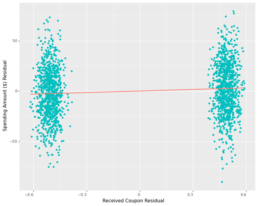
Comparing the variance of the original spending amount to that of the residuals of the spending amount confirms that we are able to achieve a more than 80% reduction in variance.

print("Spending Amount Variance:", round(np.var(data["Y"]),2))
print("Spending Amount Residual Variance:", round(np.var(residuals["res_y"]),2))

Due to the mechanics of regression, we can obtain the same result by regressing the residuals of the spending amount against the residuals of the treatment:

model_res = smf.ols('res_y ~ res_t', data=residuals).fit()
model_res.summary().tables[1]

Conclusion

Applying a simple regression adjustment to our experiment analysis can go a long way in reducing the variance of our outcome metric, which can be particularly helpful if we are trying to detect a small effect in our experiment. In part 2 of this series we will do a deep dive into finding out the performances of various methods in this space. Specifically, we will be running simulations with varying degrees of complexities in the data generating process and applying MLRATE - machine learning regression-adjusted treatment effect estimator, the latest invention in this space, as well as other methods such as CUPED and regression adjustment. Stay tuned.

Code

The original notebook can be found in my repository.