Variance Reduction in Experiments, Part 2 - Covariance Adjustment Methods

Difference-in-means (DIM)

DIM is a simple and consistent estimate of the ATE and will be the baseline in our analysis since it does not involve any covariate adjustment:

\[\hat{\tau}_{DIM} = \frac{1}{n_T}\sum_{i\in T}Y_i - \frac{1}{n_C}\sum_{i\in C}Y_i\]

Regression adjustment (OLS_adj)

This is the coefficient estimate of the treatment indicator, \(T\), which is 1 if unit \(i\) is in treatment and 0 otherwise, from the outcome regression that includes covariates, \(X\), in a linear and additive manner, and assumes a constant treatment effect across all units:

\[Y_i = \beta_0 + \tau T_i + \beta X_i + \epsilon_i\] To see why the OLS estimator of \(\tau\) is a consistent estimator of the ATE, let’s consider the regression function for treated and control separately and then take the difference:

\[ \begin{align*} E[Y|T,X] &= \beta_0 + \tau T + \beta X \\ E[Y|T=1,X] &= \beta_0 + \tau T + \beta X\\ E[Y|T=0,X] &= \beta_0 + \beta X\\ E[Y|T=1,X] - E[Y|T=0,X] &= \tau(x) = \tau \end{align*} \]

It follows that:

\[ATE = E[E[Y|T=1,X] - E[Y|T=0,X]] = E[\tau] = \tau\]

Regression adjustment with interactions (OLS_int)

This is the coefficient estimate of the treatment indicator, \(T\), from the outcome regression that includes not only covariates, \(X\), but also interactions between \(T\) and the demeaned covariates.

Contrary to OLS_adj, here we do not assume the effect is constant across all units, rather we allow the treatment effect to vary with the covariates, albeit in a linear and additive way.

\[Y_i = \beta_0 + \tau T_i + \beta X_i + \alpha T_i(X_i - \bar{X_i}) + \epsilon_i\] The OLS estimator of \(\tau\) once again is a consistent and asymptotically normal estimator of the ATE. To see why, let’s again take the regression function for treated and control separately and then take the difference:

\[ \begin{align*} E[Y|T,X] &= \beta_0 + \tau T + \beta X + \alpha T_i(X_i - \bar{X_i}) \\ E[Y|T=1,X] &= \beta_0 + \tau T + \beta X + \alpha T(X - \bar{X}) \\ E[Y|T=0,X] &= \beta_0 + \beta X\\ E[Y|T=1,X] - E[Y|T=0,X] &= \tau(x) = \tau + \alpha T(X - \bar{X}) \end{align*}\] So, we have:

\[\begin{align*} ATE &= E[\tau(x)] = E[E[Y|T=1,X] - E[Y|T=0,X]]\\ ATE &= E[\tau + \alpha (X - \bar{X})]\\ ATE &= \tau + \alpha \underbrace{E[X - \bar{X}]}_0\\ ATE &= \tau \end{align*}\]

Controlled-experiment using pre-experiment data (CUPED)

CUPED (Deng et al., 2013) rests on the idea of using a pre-experiment covariate, \(X\), that is highly correlated with the outcome, \(Y\), but is unrelated to the treatment, \(T\). The pre-experiment value of the outcome, \(Y\), is a natural candidate as it meets these criteria. Conditional on having access to such a covariate in our data, we apply CUPED as follows:

1. Obtain \(\theta\):

\[\theta = cov(Y,X)/var(X)\]

2. Create a transformed outcome, \(Y_{cuped}\), for each unit \(i\):

\[Y_{cuped} = Y - \theta(X - mean(X))\]

3. Estimate \(\tau\) from:

\[Y_i = \beta_0 + \tau T_i + \epsilon_i\] This way the variance of \(Y\) is reduced by \(1-Corr(X, Y)\):

\[Var(Y_{cuped}) = Var(Y)(1-Corr(Y,X))\] In our simulations, we designed \(X_1\) in all experiment data such that it satisfies the criteria mentioned above.

Difference-in-differences (DID)

The DID estimator in the context of covariate adjustment is not to be confused with the DID estimator used in panel data applications. DID in this context is obtained by first training a machine learning model \(g(X)\) for predicting \(Y\) from \(X\), and then computing the difference between the treatment and control group averages of \(Y − g(X)\) (Yongyi et al., 2021).

The motivation behind DID is that because \(g(X)\) and \(T\) are independent, the resulting estimator has the same expectation as the DIM estimator:

\[E[Y - g(X)|T=1] - E[Y - g(X)|T=0] = E[Y|T=1] - E[Y|T=0]\] However, if \(g(X)\) is a good predictor of \(Y\) then \(Var(Y)\) will exceed \(Var(Y − g(X))\), and the DID estimate based on averages of \(Y −g(X)\) will have lower variance than the DIM estimate based on averages of \(Y\).

Furthermore, using machine learning allows us to capture complex interplay between the outcome and the covariates in a data-driven way without relying on functional form assumptions as we do in OLS_adj and OLS_int.

A critical point is to use cross-fitting. Simply put, we split the data into 2 parts, use one part to build \(g(X)\) and use the other part to obtain predictions and repeat the process by exchanging the parts. We end up with predictions for every observation that are generated by a model trained only on other observations. In this analysis we apply cross-fitting for both DID and MLRATE, since both use machine learning predictions in the final estimator, but the original paper applies it only for MLRATE (Yongyi et al., 2021).

DID is obtained as follows:

1. Train \(g(X)\) by using cross-fitting and predicting \(Y\) from \(X\).

2. Create \(Y_res\) for each unit \(i\):

\[Y_{res} = Y - g(X)\]

3. Estimate \(\tau\) from:

\[\hat{\tau}_{DID} = \frac{1}{n_T}\sum_{i\in T}Y_{i_{res}} - \frac{1}{n_C}\sum_{i\in C}Y_{i_{res}}\]

Machine learning regression-adjusted treatment effect estimator (MLRATE)

The main difference between DID and MLRATE is that instead of directly subtracting the machine learning predictions \(g(X)\) from the outcome \(Y\), it includes the predictions as well as the interactions between \(T\) and the demeaned predictions as regressors in a subsequent linear regression step (Yongyi et al., 2021).

MLRATE proceeds as follows:

1. Train \(g(X)\) by using cross-fitting and predicting \(Y\) from \(X\).

2. Obtain \(\tau\) estimate:

\[Y_i = \beta_0 + \tau T_i + \beta g(X_i) + \alpha T_i(g(X_i) - g(\bar{X_i}) + \epsilon_i\] It is shown that including predictions as regressors guarantees robustness of the estimator to poor predictions, and MLRATE has an asymptotic variance no larger than the DIM estimator.

def mlpredict(dfml,p):
    XGB_reg = XGBRegressor(learning_rate = 0.1, 
                            max_depth = 6, 
                            n_estimators = 500, 
                            reg_lambda = 1)

    X_mat = dfml.columns.tolist()[0:p]
    
    kfold = StratifiedKFold(n_splits=2, shuffle=True, random_state=1)

    ix = []
    Yhat = []
    for train_index, test_index in kfold.split(dfml, dfml["T"]):
        
        df_train = dfml.iloc[train_index].reset_index()
        df_test = dfml.iloc[test_index].reset_index()

        X_train = df_train[X_mat].copy()
        y_train = df_train['Y'].copy()
        X_test =  df_test[X_mat].copy()
        
        XGB_reg.fit(X_train, y_train)

        Y_hat = XGB_reg.predict(X_test)

        ix.extend(list(test_index))
        Yhat.extend(list(Y_hat))

    df_ml = pd.DataFrame({'ix':ix,'Yhat':Yhat}).sort_values(by='ix').reset_index(drop=True)
    df_ml[['Y','T']] = dfml[['Y','T']]
    df_ml['Ytilde'] = df_ml['Yhat'] - np.mean(df_ml['Yhat'])
    df_ml['Yres'] = df_ml['Y'] - df_ml['Yhat']
    df_ml = df_ml.drop('ix', axis=1)

    return df_ml

Data Generating Process (DGP)

To compare the effectiveness of these 5 covariate adjustment methods in reducing variance under varying degrees of complexities, we have a DGP that has \(N = 2000\) iid observations and 10 covariates distributed as \(N(0,I(10×10))\). The treatment indicator is \(T_i ∼ Bernoulli(0.5)\), and the error term is distributed as \(N(0,25²)\). Treatment is independent of covariates and the error term, which itself is independent of the covariates. The outcome \(Y_i\) and the treatment effect function \(\tau(X_i)\) depend on the functional forms as follows:

1. Linear Effects of Covariates & Constant Treatment Effect

\[\begin{align*} Y_i &= 225+ \tau(X_i)T_i+50X_{i1}+5X_{i2}+20(X_{i3}−0.5)+10X_{i4}+5X_{i5}+\epsilon_i\\ \tau(X_i) &= 5 \end{align*}\]

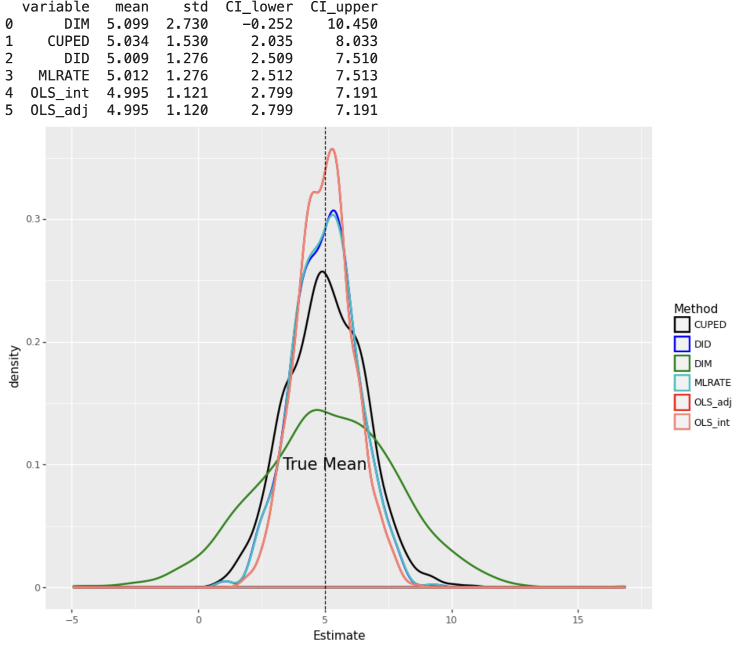
2. Linear Effects of Covariates & Varying Treatment Effect

\[\begin{align*} Y_i &= 225+ \tau(X_i)T_i+50X_{i1}+5X_{i2}+20(X_{i3}−0.5)+10X_{i4}+5X_{i5}+\epsilon_i\\ \tau(X_i) &= 5X_{i1} + 5log(1+exp(X_{i2})) \end{align*}\]

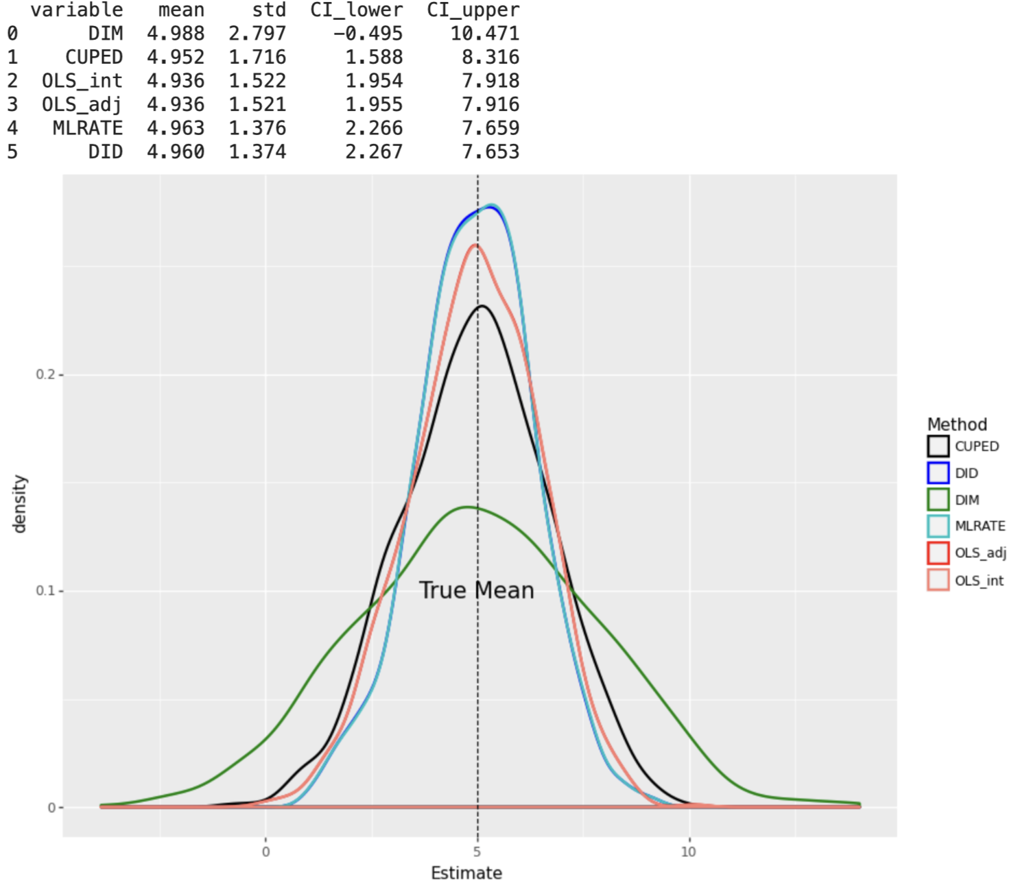
3. Non-linear Effects of Covariates & Constant Treatment Effect

\[\begin{align*} Y_i &= 225+ \tau(X_i)T_i+50X_{i1}+5sin(\pi X_{i1}X_{i2}) + 10(X_{i3}−0.5)^2+10X_{i4}^2+5X_{i5}^3+\epsilon_i\\ \tau(X_i) &= 5 \end{align*}\]

4. Non-linear Effects of Covariates & Varying Treatment Effect

\[\begin{align*} Y_i &= 225+ \tau(X_i)T_i+50X_{i1}+5sin(\pi X_{i1}X_{i2}) + 10(X_{i3}−0.5)^2+10X_{i4}^2+5X_{i5}^3+\epsilon_i\\ \tau(X_i) &= 5X_{i1} + 5log(1+exp(X_{i2})) \end{align*}\]

def dgp(n=2000, p=10, linear=True, constant=True):
        
    Xmat = np.random.multivariate_normal(np.zeros(p), np.eye(p), size=n).astype('float32')

    T = np.random.binomial(1, 0.5, n).astype('int8')

    col_list = ['X' + str(x) for x in range(1,(p+1))]

    df = pd.DataFrame(Xmat, columns = col_list)
    
    # functional form of the covariates
    if linear:
        B = 225 + 50*df['X1'] + 5*df['X2'] + 20*(df['X3']-0.5) + 10*df['X4'] + 5*df['X5']
    else:
        B = 225 + 50*df['X1'] + 5*np.sin(np.pi*df['X1']*df['X2'] ) + 10*(df['X3']-0.5)**2 + 10*df['X4']**2 + 5*df['X5']**3
    
    # constant ate or non-constant
    tau = 5 if constant else 5*df['X1'] + 5*np.log(1 + np.exp(df['X2']))
    
    Y = (B + tau*T + np.random.normal(0,25,n)).astype('float32')
        
    df['T'] = T
    df['Y'] = Y    
    return df

We generate 1000 datasets under each functional form and apply each covariate adjustment method to these data.

def experiment(**kwargs):
    
    dct = {}
    
    n = kwargs['n']
    p = kwargs['p']
    linear = kwargs['linear']
    constant = kwargs['constant']
    
    df = dgp(n,p,linear,constant)
    
    #1. Difference-in-means
    mu_treated = np.mean(df.query('T==1')['Y'])
    mu_control = np.mean(df.query('T==0')['Y'])
    
    dct['DIM'] = mu_treated - mu_control
    
    #2. OLS adjusted
    if kwargs['OLS_adj']:
        
        ols_adj = smf.ols('Y ~' + ('+').join(df.columns.tolist()[0:(p+1)]),
                 data = df).fit(cov_type='HC1',use_t=True)

        dct['OLS_adj'] = ols_adj.params['T']
    
    #3. OLS interacted
    if kwargs['OLS_int']:
        df = df.assign(**({c+'tilde': (df[c] - df[c].mean()) for c in df.columns.tolist()[0:p]}))
    
        ols_int = smf.ols('Y ~' + ('+').join(df.columns.tolist()[0:(p+1)]) + '+' + 'T:('+('+').join(df.columns.tolist()[p+2:])+')',
                 data = df).fit(cov_type='HC1',use_t=True)

        dct['OLS_int'] = ols_int.params['T']
    
    #4. CUPED
    if kwargs['CUPED']:
        theta = smf.ols('Y ~ X1',data = df).fit(cov_type='HC1',use_t=True).params['X1']

        df['Y_res'] = df['Y'] - theta*(df['X1'] - np.mean(df['X1']))
        
        cuped = smf.ols('Y_res ~ T', data=df).fit(cov_type='HC1',use_t=True)

        dct['CUPED'] = cuped.params['T']
        
    pred_df = mlpredict(df,p)

    #5. Difference-in-differences
    if kwargs['DID']:
        mu2_treated = np.mean(pred_df.query('T==1')['Yres'])
        mu2_control = np.mean(pred_df.query('T==0')['Yres'])

        dct['DID'] = mu2_treated - mu2_control

    #6. MLRATE
    if kwargs['MLRATE']:
        mlrate =  smf.ols('Y ~ T + Yhat + T:Ytilde',
                     data = pred_df).fit(cov_type='HC1',use_t=True)

        dct['MLRATE'] = mlrate.params['T']
    
    return dct

Finally, we print the estimates, their standard errors and the 95% confidence intervals as well as plot the distributions.

def plot_experiment(results, constant = True ):
    
    results_long = pd.melt(results, value_vars=results.columns.tolist() )
    
    print(round(results_long.groupby('variable').agg(mean=("value", "mean"), std=("value", "std"))
          .reset_index().sort_values(by='std', ascending=False).reset_index(drop=True)
          .assign(CI_lower= lambda x: x['mean'] - x['std']*1.96,
                CI_upper= lambda x: x['mean'] + x['std']*1.96,),3)
         )
        
    mu = 5 if constant else 4
    
    p = (ggplot(results_long, aes(x='value',color='variable') ) + 
     geom_density(size=1 )+
     scale_color_manual(values = ['black', 'blue', 'green', 'c','red', 'salmon', 'magenta' ]) + 
     geom_vline(xintercept=mu, colour='black', linetype='dashed' ) + 
     annotate("text", x=mu, y=.1, label="True Mean", size=15)+
     labs(color='Method')  +
     xlab('Estimate') +
     theme(figure_size=(10, 8))
    )
    
    print(p)

Findings

The simulation results are shown in the figures below and the key findings are as follows:

1. Every covariate adjustment method achieves smaller standard errors than the DIM estimator regardless of the DGP, however, the degree of reduction depends on the complexity of the DGP.

2. When the DGP consists of linear effects of covariates, the OLS_adj and OLS_int estimators have the smallest standard errors, under both constant and varying treatment effects.

3. When the DGP consists of non-linear effects of covariates, machine learning based estimators DID and MLRATE have the smallest standard errors, under both constant and varying treatment effects.

4. Since non-linearity in covariates and varying treatment effects are both the norm rather than the exception in real-life applications, we conclude that machine learning based adjustment methods are superior than other methods in reducing variance in experiments.

5. Finally, CUPED underperforms other methods under every scenario. This is mainly because the original version of CUPED uses a single covariate for adjustment and that’s how we implement it. It is possible to extend CUPED for multiple covariates.

%%time
tqdm._instances.clear() 
sim = 1000

results1 = Parallel(n_jobs=8)(delayed(experiment)(n=2000, p=10, linear=True, constant=True,
                                    OLS_adj=True, OLS_int=True, CUPED=True, DID=True, MLRATE=True)\
                                    for _ in tqdm(range(sim)) )

results_df1 = pd.DataFrame(results1)

plot_experiment(results_df1)

results2 = Parallel(n_jobs=8)(delayed(experiment)(n=2000, p=10,linear=True, constant=False,
                                    OLS_adj=True, OLS_int=True, CUPED=True, DID=True, MLRATE=True)\
                                    for _ in tqdm(range(sim)) )

results_df2 = pd.DataFrame(results2)

plot_experiment(results_df2, False)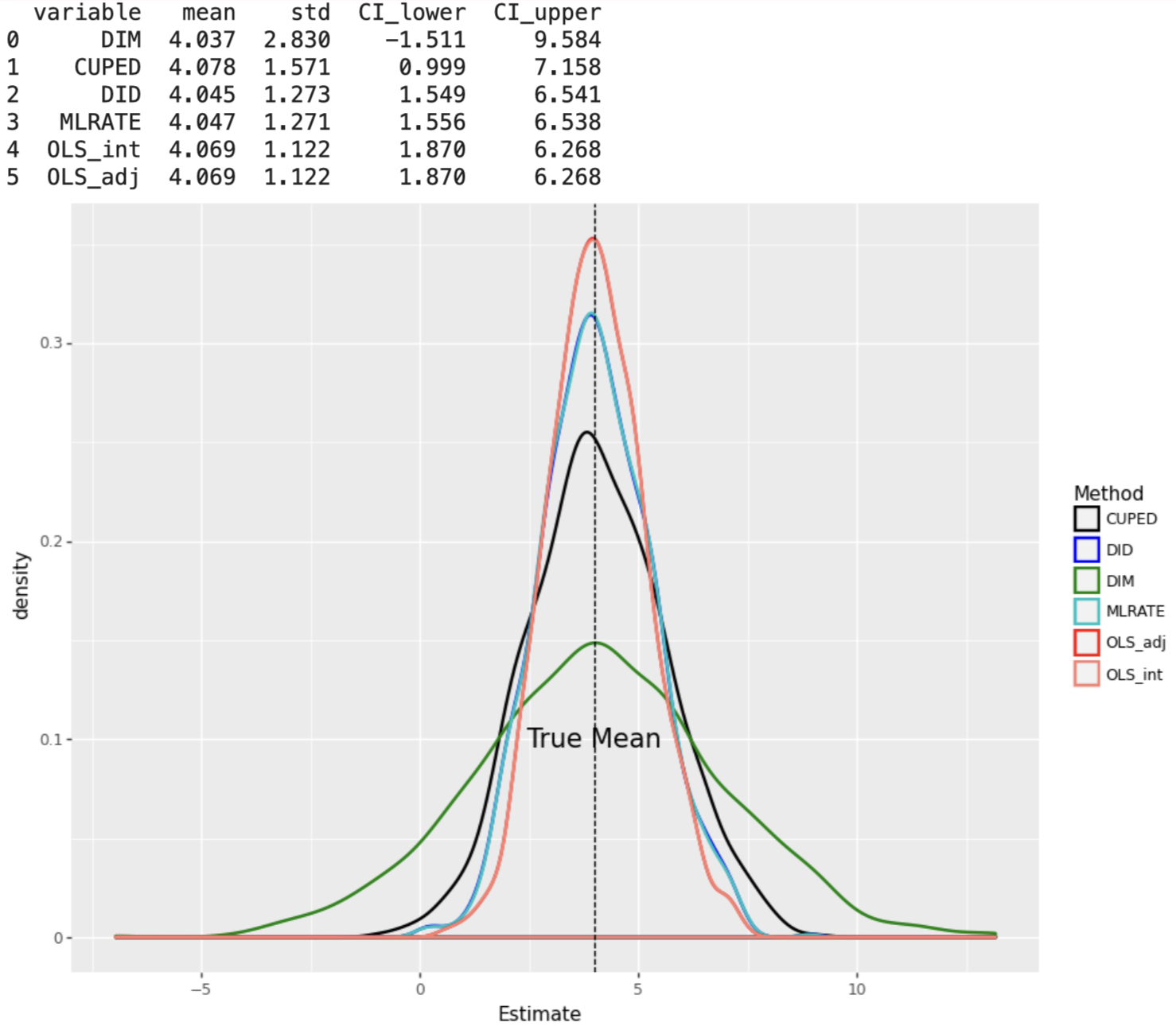

results3 = Parallel(n_jobs=8)(delayed(experiment)(n=2000, p=10,linear=False, constant=True,
                                    OLS_adj=True, OLS_int=True, CUPED=True, DID=True, MLRATE=True)\
                                    for _ in tqdm(range(sim)) )

results_df3 = pd.DataFrame(results3)

plot_experiment(results_df3)

results4 = Parallel(n_jobs=8)(delayed(experiment)(n=2000, p=10,linear=False, constant=False,
                             OLS_adj=True, OLS_int=True, CUPED=True, DID=True, MLRATE=True)\
                             for _ in tqdm(range(sim)) )

results_df4 = pd.DataFrame(results4)

plot_experiment(results_df4, False)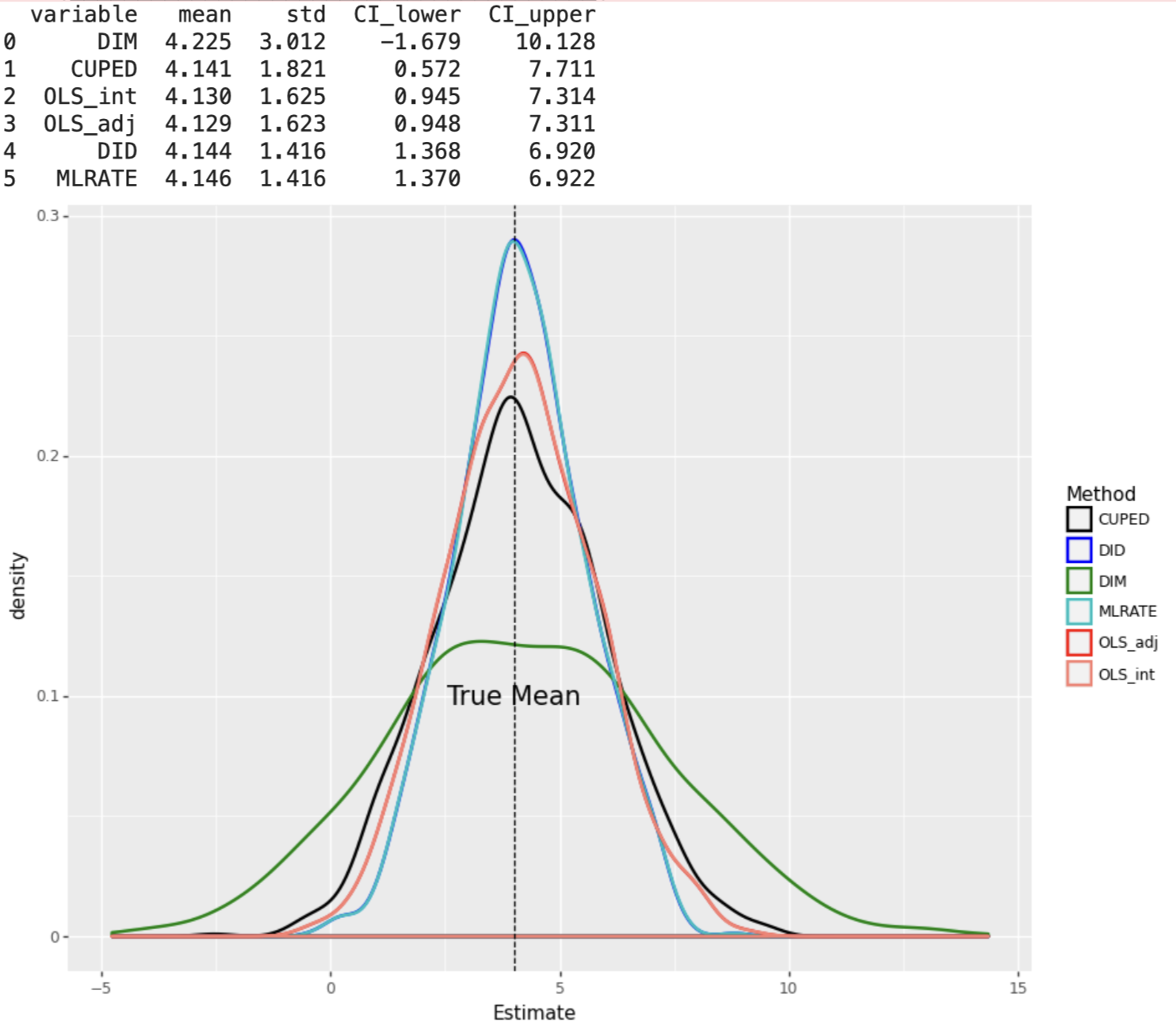

Conclusion

This concludes the two-article series on variance reduction in experiments. In part 1 we built an intuition towards the importance of variance reduction in experiments and in part 2 we have analyzed different covariate adjustment methods. We have seen that all of the methods result in tighter confidence intervals than the simple DIM estimator. As such, covariate adjustment should become a standard practice when analyzing experiments. When it comes to which method to apply, we have seen that machine learning based estimators perform best especially when there is complex interplay in the DGP, which certainly is a more realistic representation of the real-world.

Code

The original notebook can be found in my repository.

References

[1] W. Lin, Agnostic notes on regression adjustments to experimental data: Reexamining freedman’s critique. (2013), The Annals of Applied Statistics.

[2] A. Deng, Y. Xu, R. Kohavi, T. Walker, Improving the Sensitivity of Online Controlled Experiments by Utilizing Pre-Experiment Data (2013), WSDM.

[3] G. Yongyi, C. Dominic, M. Konutgan, W. Li, C. Schoener, M. Goldman, Machine Learning for Variance Reduction in Online Experiments (2021), NeurIPS.